现代机器人学: 旋量法推导机器人运动学与动力学方程
本文公式可能有误,欢迎评论指正
刚体构型描述,旋量方法
斜对称矩阵(Skew symmetric)
a×b=[a]b
[a]≜⎣⎡0a3−a2−a30a1a2−a10⎦⎤
特殊正交群(Special Orthogonal Group)
SO(n)={R∈Rn×n:RTR=I,det(R)=1}ARB: orientation of {B} relative to {A} expressed in {A} frame
对于绕轴旋转运动, 设单位转轴ω, 旋转矩阵R可以通过罗德里格斯公式计算:
由微分方程
q˙(t)=ω×q(t)=[ω]q(t)
可得
q(t)=e[ω]tq(0)
因而
Rot(ω,θ)=e[ω]θ==I+[ω]sinθ+[ω]2(1−cosθ)
[ωs(t)]=R˙s(t)Rs−1(t)
特殊欧几里得群(Special Euclidean Group)
se(3)={([ω],v):[ω]∈so(3),v∈R3}
Homogeneous Transformation Matrix:
ATB=(R,p)=[ARB0ApB1]
T−1=[R0p1]−1=[RT0−RTp1]
R[w]RT=[Rw]
[S]=(ω,v)=[[ω]0v0]
p~(t)=e[S]tp~(0),e[S]t∈SE(3)
正向运动学
运动旋量Twist
AV=AXBBV
AXB=[AdT]≜[R[p]R0R]
[Vb]=T−1T˙,[Vs]=T˙T−1
如果坐标系不动,则先求导再坐标变换与先坐标变换再求导等价: o[dtd(r)]=dtd(or)
, 也即or˙=or˚
如果坐标系移动,则有: o[dtd(r)]=dtd(or)+BωB×or
PoE
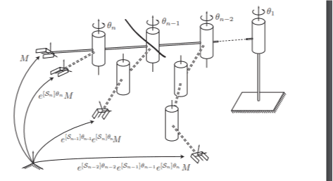
PoE需要从end effector的位置和姿态开始,向base的位置和姿态推导,
这样可以避免靠近base的关节的运动影响到靠近end effector的轴的位置和姿态。
当然,前向和后向最后可以证明是一样的,没有区别,但是前向的PoE需要考虑到上面的问题,导致求解比较麻烦.
雅可比矩阵
Geometric Jacobian
对于n轴robot,令V为end-effector的twist, J为雅可比矩阵, J_i为第i个关节的雅可比矩阵, coordinate free形式下有:
V=J(θ)θ˙=J1(θ)θ1˙+⋯+Jn(θ)θ˙n
因此有Ji(θ)=Si(θ)
考虑到坐标变换有
J(θ)=[S1,[AdT(θ1)]Sˉ2]
也即0Ji(θ)=0Xi(θ)iSi
Analytical Jacobian
定义:对于一个机器人,其末端执行器的位置和姿态可以用一个向量表示,这个向量的每个元素是末端执行器的位置和姿态的一个分量。这个向量的导数就是机器人的雅可比矩阵。
注意:x可能为6维向量,分别为位置和姿态的三个分量,也可能仅仅是位置的三维向量。
对于末端执行器位置与姿态向量p(θ),
J=⎣⎡∂θA∂px∂θA∂py∂θA∂pz∂θB∂px∂θB∂py∂θB∂pz∂θC∂px∂θC∂py∂θC∂pz⎦⎤
动力学
加速度的旋量表示
对于q¨(t)=v˙o(t)的证明:
由q˙(t)=v0(t)+w(t)×q(t)
求导可得,q¨(t)=v˙0(t)+w˙(t)×oq(t)+w(t)×q˙(t),证得结论.
由AXB=[AdT]≜[R[p]R0R],
可得AXB˙=dtd([R[p]R0R])
其中,([p]R)′=[p˙]R+[p]R˙
[p˙]=[v0+w×p]=[v0]+[w×p]=[v0]+[w][p]−[p][w]
其中,对于, [w×p]=[w][p]−[p][w]部分,
李括号性质的分析与证明中有详细证明
因此有AXB˙=[[w]R[v0]R+[w][p]R0[w]R]=[[w][v0]0[w]]AXB
对于V1×V2,令其等于[V1×]V2(一种李括号)
则有[V1×]≜[[w][v]0[w]]
代入之前的式子,有AXB˙=[VB×]AXB
空间加速度(spatial acceleration): A=V˙=[ω˙v˙o]
根据定义o(Abody)=dtd(oVbody)=dtd(oXBoVbody)=oX˙BBVbody+oXBBV˚body
因此o(Abody)=[oVB×]oXBBVbody+oXBBV˚body
加速度坐标变换: BA=BX0∘A
力的旋量表示
对于O点力矩nO, 有n0=∑iopi×fi
空间力(Spatial Force),也称力旋量(Wrench): F=[nOf]
frame A下有AF=[AnoAAf]
空间力坐标变换: AF=AXB∗BF, 其中AXB∗=BXAT的证明:
又易证X˙B∗=[V×∗]XB∗,其中[V×∗]=[[w]0[v][w]]
可推导空间力的导数: A[dtdF]=dtd(AF)+[AV×∗]AF
[AnOAAf]=[ARB0−ARB[BPA]ARB][BnOBBf]
[ARB0−ARB[BPA]ARB]=[BRA[BPA]BRA0BRA]T=BXAT
power: P=(AV)TAF
由V=S^θ˙(S^为screw axis of the joint)
并定义torque,τ=S^TF=FTS^(由几何雅可比J(θ)=S(θ)可得τ=J(θ)^TF=FTJ(θ)^)
可得,P=VTF=(S^TF)θ˙≜τθ˙
转动惯量Iˉ=∫Vρ(r)[r][r]Tdr,特别地,对于原点恰在质心的情况,转动惯量为常量
对于线性动量(linear momentum),L=mv
可推得角动量(angluar momentum):ϕ=r×L=r×(mω×r)=m[r][−r]ω=Iˉω
空间动量(spatial momentum):h≜[ϕnL]
空间动量坐标变换:Ah=AXB∗Bh
同空间力的推导一样,也可以推导空间动量的导数: A[dtdh]=dtd(Ah)+[AV×∗]h
令h=IV,其中I为空间惯量矩阵
对于frame C,如果原点恰为质心,则空间惯量CI=[cIˉc00mI3]
空间惯量坐标变换:AI=AXC∗CICXA
newton-euler方程
newton-euler方程: F=dtdh=IA+V×∗IV
证明: oF=o(dtdh)=dtd(oh)=dtd(oIoV)
=oI˙∘V+oIoA
=dtd(oXB∗BIBX0)oV+oIoA
其中,dtd(oXB∗BIBX0)oV
=oXB˙∗BIBXooV+oXB∗BIBXo˙oV
由于oXBBXo=I(I为单位矩阵)
有oXB˙BXo+oXBBXo˙=0
因此有oXB˙=−oXBBXo˙oXBB
因此dtd(oXB∗BIBX0)oV
=[oVB×∗]oXB∗BIBXooV−oXB∗BIBXo[oVB×]0V
=[oVB×∗]oXB∗BIBXooV−0
于是证得newton-euler方程
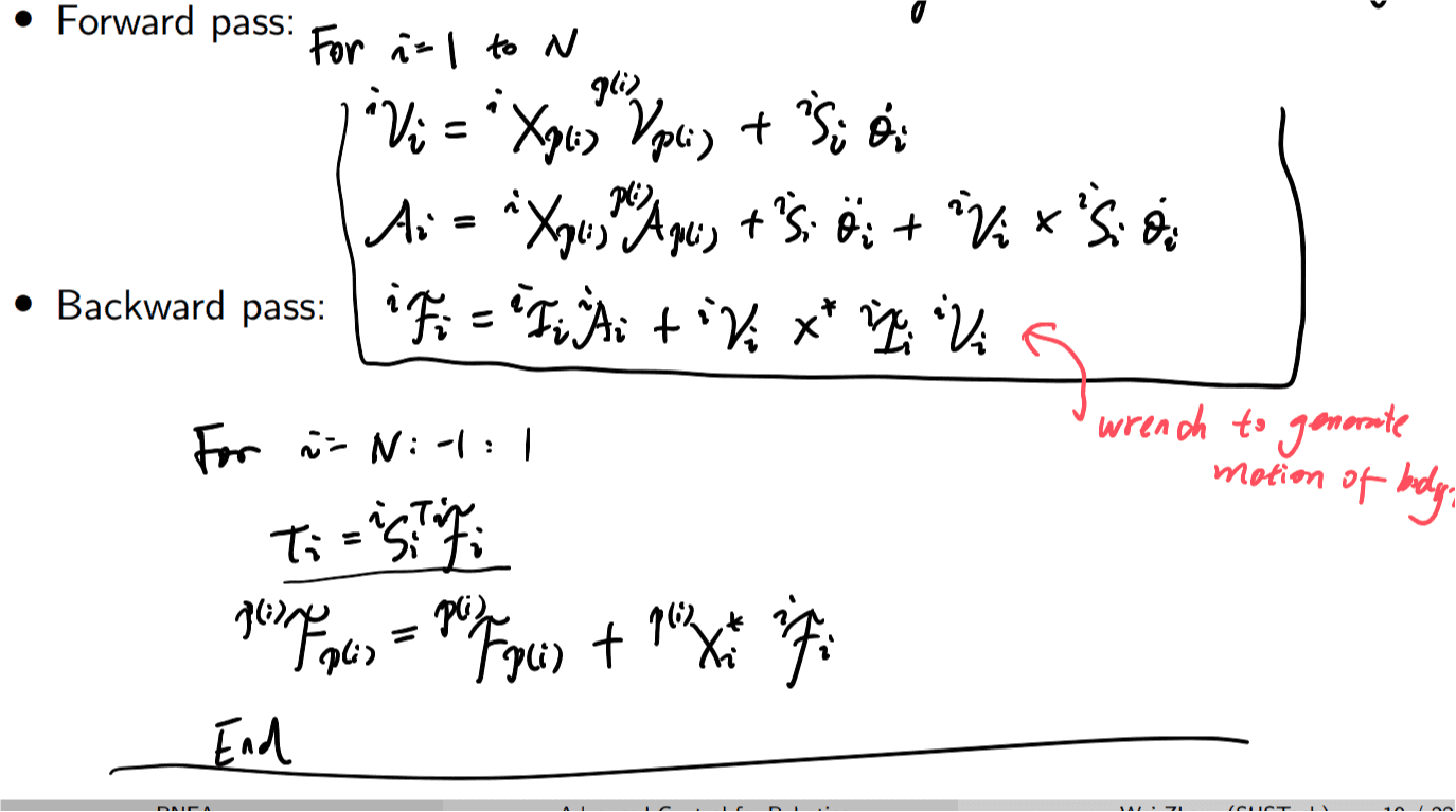
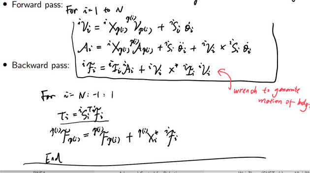
Recursive Newton-Euler:
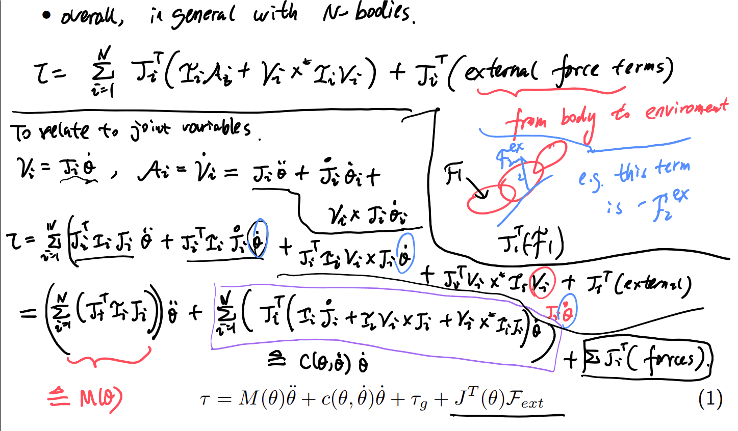
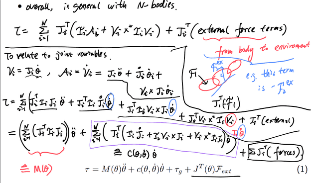
拉格朗日方程
τ=M(θ)θ¨+c~(θ,θ˙)
证明如下图:
参考
南科大高等机器人控制 课程官网
知乎: 控制门下一走狗
刚体运动与旋量入门
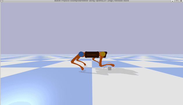
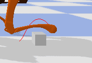
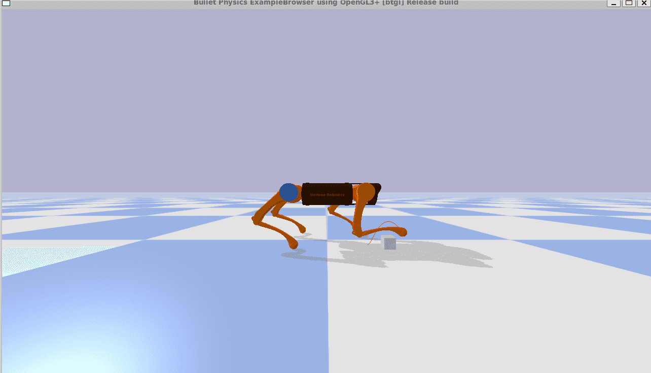
pybullet仿真与轨迹显示
使用多项式方式平滑轨迹
控制方式基于Raibert's formula
τhip=kp(ϕdes−ϕ)+kν(ϕ˙des−p˙hi)